The Art of JPEG

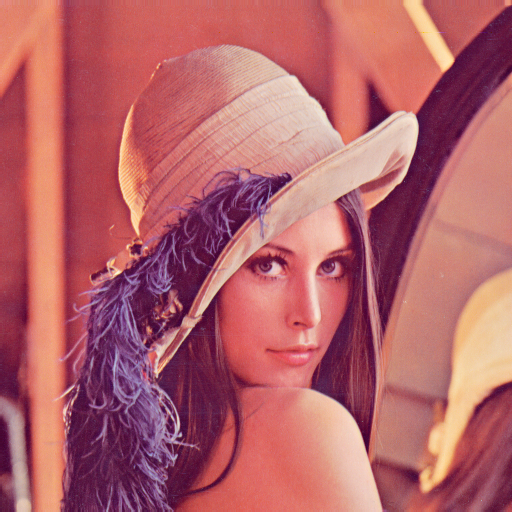
The famous Lenna image, often used in image processing research. A fun fact that many developers may have missed: it was cropped from a Playboy magazine centerfold in 1972. The image has become a standard test image in the field of image processing, and today, we will use it to explore how JPEG works.

Feel free to upload your own image using the file input below the picture!

Size in pixels:: 0 x 0
Size in kilobytes:: 0
Unique colors:: 0

1^st❖ Color Space Conversion

JPEG starts with a color space conversion from RGB to YCbCr. This separates the image into one luminance (Y) and two chrominance (Cb and Cr) components. The human eye is more sensitive to luminance than chrominance, allowing JPEG to compress the chrominance channels more aggressively without significant perceived loss in quality.

Chrominance Threshold:Chrominance Amplify:

The images above show the Y, Cb, and Cr channels extracted from the original image. The sliders allow you to adjust the threshold and amplification for the chrominance channels and are for visualization purposes only.

2^nd❖ Chroma Subsampling

After color space conversion, JPEG typically applies chroma subsampling. This reduces the resolution of the chrominance channels (Cb and Cr) relative to the luminance channel (Y). Common subsampling ratios include 4:4:4 (no subsampling), 4:2:2, and 4:2:0. By reducing the amount of chrominance data, JPEG can achieve significant compression while maintaining visual quality.

Subsampling Amount:

The images above illustrate the effect of chroma subsampling on the Cb and Cr channels. Notice how the resolution is reduced, which contributes to overall file size reduction in JPEG compression.

3^rd❖ Discrete Cosine Transform

The Discrete Cosine Transform (DCT) is a mathematical operation that transforms spatial domain data (pixel values) into frequency domain data. In JPEG, the image is divided into 8x8 pixel blocks, and each block undergoes DCT. This transformation helps to separate the image into parts of differing importance with respect to human perception.

8x8 Pixel Grid Overlay — Hover or click to zoom into an 8x8 block

Zoomed-in 8x8 Block — Zoomed-in view of selected 8x8 block

Frequency Patterns Table — Frequency patterns in an 8x8 DCT block

Presence of frequency table

16	11	10	16	24	40	51	61
12	12	14	19	26	58	60	55
14	13	16	24	40	57	69	56
14	17	22	29	51	87	80	62
18	22	37	56	68	109	103	77
24	35	55	64	81	104	113	92
49	64	78	87	103	121	120	101
72	92	95	98	112	100	103	99

Standard JPEG Quantization Table. There are many.

Quantized DCT Coefficients

4^th❖ Entropy Coding

Look at the red zig-zag line in the last table, it shows the order in which the quantized DCT coefficients are read for entropy coding. This ordering helps to group low-frequency coefficients (which are more likely to be non-zero) together, followed by high-frequency coefficients (which are more likely to be zero). This arrangement is beneficial for the subsequent entropy coding step, as it increases the efficiency of compression algorithms like Huffman coding or arithmetic coding.

Before Entropy Coding

After Entropy Coding

Huffman Codes

{}

Encoded Hex String

Block Level Compression Ratio

Summary

In summary, JPEG compression is a complex process that involves several stages, each contributing to the overall reduction in file size while striving to maintain visual quality. Understanding these processes not only provides insight into how digital images are stored and transmitted but also highlights the ingenuity behind one of the most widely used image formats in the world.

I hope you enjoyed this deep dive into the art of JPEG!